Introduction
========================================================================
Image filtering techniques such as Gaussian smoothing and linear and
nonlinear diffusion all have a local smoothing that is the same in all directions,
_i.e._ it is isotropic.
By introducing an anisotropic diffusivity the smoothing can be directed along
image features such that they are coherently smeared or even enhanced, see **Figure 1**.
In this blog post I will derive and show how nonlinear anisotropic diffusion for
coherence enhancing image smoothing can be implemented in python.
[In a previous post](../image_smoothing_by_nonlinear_diffusion) I showed how isotropic nonlinear diffusion can be used
for feature preserving image filters and this is for all intents and purposes
a direct continuation of that approach.
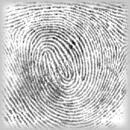
a) Original.
b) Video transition.

c) Result.
**Figure 1:** _Anisotropic filtering can be used to enhance coherent structures such as fingerprints. The video in the middle transforms from the unfiltered image on the left to the filtered image on the right. The original fingerprint image on the left is taken from [#weickert1998]._
The anisotropic image filtering methods emerged in the 1990s and the defacto work was summarized
by Joachim Weickert in his 1998 monograph on anisotropic diffusion
in image processing [#weickert1998].
The text is heavy on mathematics and applications and not so much on
implementation details but I highly recommend reading it if only
the first chapter or even the first 20 pages since it covers the historical
connections to signal processing.
Though it does not cover this subject exactly I highly recommend the lecture
series on _Variational Methods for Computer Vision_ by Daniel Cremers [#cvprtum]
which is available on youtube.
A comprehensive but very theoretical review of this and related methods can
be found in the book _Mathematical problems in image processing_
[#aubertkornprobst2006].
It serves as a very good collection and contextualization of the
academic literature up to its year of publication but it does not
cover much of the numerical schemes needed to practically implement
the methods.
A much better coverage of implementation details can be found in the work by
[#kroon2009coherence]. Further, that work was released as an open source
matlab toolbox [#kroon2010toolbox]. It includes basically everything covered
in this blog post and it also has implementations for filtering
of 3D, volumetric, images.
!!! Info
_**Extending the nonlinear diffusion using anisotropic diffusivity**_
When I started to read up on this subject it became clear that was what often
called anisotropic diffusion was actually nonlinear, but isotropic,
diffusion. In order to investigate what I had originally intended, the diffusion
of long but noisy or intereupted structures as a means of repair or reconstruction,
I would have to keep investigating.
Doing so proved to be a challenging venture into partial differental equations
and finite differences.
Image smoothing by anisotropic diffusion
========================================================================
The diffusion equation and categorization
--------------------------------------------------------------------------------
As described in [my previous blog post](../image_smoothing_by_nonlinear_diffusion) the
**diffusion equation** can be formulated as a partial differential equation on the image
domain in 2D or 3D, $\Omega \in \Real^{2}$ or $\Omega \in \Real^{3}$.
\begin{equation}
\left\{
\begin{split}
& \frac{\partial u}{\partial_{t}} = \nabla \cdot (g \nabla u) \quad \text{in} \quad \Omega \\
& \frac{\partial u}{\partial N} = 0 \quad \text{on} \quad \partial \Omega \\
& u(0,\xfat) = u_{0}(\xfat)
\end{split}
\right.
\label{eq:diffeqdef}
\end{equation}
where $u$ is the image, a scalar field with a value at position $\xfat \in
\Omega$,
$u(\xfat) \in \Real$. $\partial \Omega$ denotes the boundary of the domain and
$u_{0}$ is the original image.
The rate of the diffusion is governed by the **diffusivity**, $g$, and
when categorizing different approaches of diffusion filters in image processing
we look at how the diffusivity is modeled.
!!! Warning:
**Confusion regarding nonlinearity and anisotropy**
As stated in my [previous blog post on nonlinear diffusion](../image_smoothing_by_nonlinear_diffusion)
there has been some confusion regarding the terminology and the
difference between nonlinear and anisotropic.
Diffusion is categorized depending on the diffusivity $g$:
1. $g = 1$ or any constant, $g \in \Real$, is called **_linear_**, **_isotropic_** and
**_homogeneous_** diffusion.
2. $g = g(\textbf{x})$ such that the amount of diffusivity depends on spatial
position is called **_inhomogeneous_**.
3. $g = g(u)$ is called **_nonlinear_** since the equation is no longer linear in
$u$.
4. $g$ is matrix valued, $D$, such that the diffusivity is not the same in different
directions. This is **_anisotropic_** diffusion. If the diffusivity depends
spatially on the diffused substance itsel, $g = g(u(\xfat)) = D(u, \xfat)$, the process
is a **_nonlinear and anisotropic_** diffusion. This is what is covered in
this blog post.
So in the anisotropic case the diffusivity is in fact a matrix valued function
with the coordinates of the image domain and the image itself as input.
\begin{equation}
D = D(u, \xfat) = g(u(\xfat)) , \quad
D =
\begin{pmatrix}
a & b \\
c & d
\end{pmatrix}
\end{equation}
Anisotropic diffusion by Weickert
-------------------------------------------------------------------------------
Just as in the nonlinear smoothing the anisotropic image filter depends on how
we choose to model the diffusivity.
Weickert [#weickert1998] proposed two different formulations for 2D filtering that use the
local image structure tensor, $J$.
\begin{equation}
\begin{split}
J = \nabla u_{\sigma} \nabla u_{\sigma}^{\intercal} =
\begin{pmatrix}
u_{\sigma x}\\
u_{\sigma y}
\end{pmatrix}
\cdot
\begin{pmatrix}
u_{\sigma x} & u_{\sigma y}
\end{pmatrix}
=
\begin{pmatrix}
u_{\sigma_{1} x} u_{\sigma x} & u_{\sigma x} u_{\sigma y} \\
u_{\sigma y} u_{\sigma x} & u_{\sigma y} u_{\sigma y}
\end{pmatrix}
\end{split}
\end{equation}
Where the image has first been smoothed using a Gaussian convolution
$u_{\sigma} = G_{\sigma} \ast u$
and we also smooth the resulting structure tensor in the same way
$J_{\rho} = G_{\rho} \ast J$.
These low pass filterings help regularize the problem and hopefully make it less
sensitive to noise in the original image $u$.
\begin{equation}
J_{\rho} = G_{\rho} \ast J =
\begin{pmatrix}
j_{11} & j_{12} \\
j_{21} & j_{22}
\end{pmatrix}
~ , ~ j_{12} = j_{21}
\end{equation}
The diffusivity matrix, $D$, will be defined through the eigenvalues
\begin{equation}
\left\{
\begin{split}
\mu_{1} &= \frac{1}{2} \left( j_{11} + j_{22} + \sqrt{ (j_{11} - j_{22})^{2} + 4 j_{12}^{2}} \right) \\
\mu_{2} &= \frac{1}{2} \left( j_{11} + j_{22} - \sqrt{ (j_{11} - j_{22})^{2} + 4 j_{12}^{2}} \right)
\end{split}
\right.
\end{equation}
and eigenvectors parallell to
\begin{equation}
\left\{
\begin{split}
v_{1} &=
\begin{pmatrix}
v_{1_{x}} \\ v_{1_{y}}
\end{pmatrix} &=
\begin{pmatrix}
2 j_{12} \\ \hphantom{-}j_{22} - j_{11} + \sqrt{ (j_{22} - j_{11})^{2} + 4 j_{12}^{2}}
\end{pmatrix}
\\
v_{2} &=
\begin{pmatrix}
v_{2_{x}} \\ v_{2_{y}}
\end{pmatrix} &=
\begin{pmatrix}
-j_{22} - j_{11} + \sqrt{ (j_{22} - j_{11})^{2} + 4 j_{12}^{2}} \\ 2 j_{12}
\end{pmatrix}
\end{split}
\right.
\end{equation}
In order to modulate the diffusivity the eigenvalues are then set depending on
the type of smoothing we want. In 2D Weickert proposed two main forms and I also
tested a simpler image smearing approach. Kroon implemented the generalized
forms of Weickerts diffusivities and also described extensions in 3D for
a specific application in medical imaging [#kroon2009coherence].
### Weickert edge enhancing
The edge enhancing smoothing will blur the image equally in both directions if
there is no strong gradient in that region, otherwise it will reduce the amount
of blurring that takes place across the image gradient and smooth it along the
detected edge.
It is modulated by the parameter $C$, which is typically set to a fixed value.
\begin{equation}
\begin{split}
\lambda_{1} &=
\left\{
\begin{split}
1 & & \quad \text{if } \mu_{1} = 0 & \\
1 & - \text{exp}(\frac{C}{\mu_{1}^{4}}) & \quad \text{else} & \quad (C = -3.315)
\end{split}
\right. \\
\lambda_{2} &= 1
\end{split}
\end{equation}
### Weickert coherence enhancing
Cohoerence enhancing smoothing will smooth the image along strong line-like features and curves such as the
patterns in a fingerprint with some diffusion taking place across the principal direction.
It is modulated by the parameter $\alpha$.
\begin{equation}
\begin{split}
\lambda_{1} &= \alpha \\
\lambda_{2} &=
\left\{
\begin{split}
& \alpha & \quad \text{if } \mu_{1} = \mu_{2}\\
& \alpha + (1 - \alpha) \text{exp}(\frac{-1}{(\mu_{1} - \mu_{2})^{2}}) & \quad \text{else}
\end{split}
\right. \\
\end{split}
\end{equation}
### Directed image smearing
The simplest possible model is to simply smooth the image only in the dominant gradient direction.
This will smear the image along lines and edges and can be used to test the correctness of the
eigenvectors.
\begin{equation}
\begin{split}
\lambda_{1} &= 1 \\
\lambda_{2} &= 0
\end{split}
\end{equation}
Then the $D$ is set to
\begin{equation}
D =
\begin{pmatrix}
a & b \\
c & d
\end{pmatrix}
=
\begin{pmatrix}
\lambda_{1} v_{1_{x}}^{2} + \lambda_{2} v_{2_{x}}^{2} &
\lambda_{1} v_{1_{x}} v_{1_{y}} + \lambda_{2} v_{2_{x}} v_{2_{y}} \\
\lambda_{1} v_{1_{x}} v_{1_{y}} + \lambda_{2} v_{2_{x}} v_{2_{y}} &
\lambda_{1} v_{1_{y}}^{2} + \lambda_{2} v_{2_{y}}^{2}
\end{pmatrix}
\end{equation}
!!! Tip:
**Anisotropic diffusion for volumetric, 3D, images**
The extension to 3D is not as straight forward as for nonlinear
image smoothing since the anisotropy can be modeled in different
ways.
Basically it boils down to having either _line_ or _plane_ enhancements
[#kroon2009coherence] and the choice depends on the shape of the main
features of interest.
Expanding the expression into discretizable operations
-------------------------------------------------------------------------------
Direct spatial discretization of Equation [eq:diffeqdef] reportedly lead to artifacts so we expand the expression
using the product rule for the divergence as proposed by [#kroon2010optimized] and in [#wiki].
\begin{equation}
\label{eq:anisdiff}
\nabla \cdot (D \nabla u) = {\cone (\nabla \cdot D) \nabla u} + {\ctwo \trace [ D (\nabla \nabla^{\intercal} u)]}
\end{equation}
where $\trace$ is the trace matrix operation, _i.e._ the sum of the
diagonal elements.
We then expand these two terms separetely starting with
\begin{equation}
\begin{split}
{\cone
(\nabla \cdot D) \nabla u
} &=
\begin{pmatrix}
{\colorC \dx a + \dy b } \\
{\colorD \dx c + \dy d } \\
\end{pmatrix}
\nabla u
\\
&= {\colorC (\dx a + \dy b) \dx u } + {\colorD (\dx c + \dy d) \dy u}
\\
&= {\colorC (a_{x} + b_{y}) \ux } + {\colorD (c_{x} + d_{y}) \uy}
\end{split}
\label{eq:divtensor}
\end{equation}
and then
\begin{equation}
\begin{split}
{\colorB
\trace [ D (\nabla \nabla^{\intercal} u)]
}
&=
\trace \left[
\begin{pmatrix}
{\colorE a} & {\colorF b} \\
{\colorF c} & {\colorG d} \\
\end{pmatrix}
\left(
\begin{pmatrix}
\dx \\ \dy
\end{pmatrix}
\cdot
\begin{pmatrix}
\dx & \dy
\end{pmatrix}
\cdot
u
\right)
\right]
\\
&=
\trace \left[
\begin{pmatrix}
{\colorE a} & {\colorF b} \\
{\colorF c} & {\colorG d} \\
\end{pmatrix}
\left(
\begin{pmatrix}
{\colorE \dxx} & {\colorF \dxy} \\
{\colorF \dxy} & {\colorG \dyy}
\end{pmatrix}
\cdot
u
\right)
\right]
\\
&=
\trace \left[
\begin{pmatrix}
{\colorE a} & {\colorF b} \\
{\colorF c} & {\colorG d} \\
\end{pmatrix}
\cdot
\begin{pmatrix}
{\colorE \uxx} & {\colorF \uxy} \\
{\colorF \uxy} & {\colorG \uyy}
\end{pmatrix}
\right]
\\
&=
\trace \left[
\begin{pmatrix}
{\colorE a \uxx} + {\colorF b \uxy} & a \uxy + b \uyy \\
c \uxx + d \uxy & {\colorF c \uxy} + {\colorG d \uyy}
\end{pmatrix}
\right]
\\
&=
{\colorE a \uxx} + {\colorF b \uxy + c \uxy} + {\colorG d \uyy}
\\
&=
{\colorE a \uxx} + {\colorG d \uyy} + {\colorF (b+c) \uxy}
\end{split}
\end{equation}
By substituting back into Equation [eq:anisdiff] we get
\begin{equation}
\label{eq:analytical}
\nabla \cdot (D \nabla u) = {\colorC (a_{x} + b_{y}) \ux} + {\colorD (c_{x} + d_{y}) \uy} + {\colorE a \uxx} + {\colorG d \uyy} + {\colorF (b+c) \uxy}
\end{equation}
!!! Info:
**Divergence of a tensor**
In Equation [eq:divtensor] we need to calculate the divergence of the tensor _D_.
Using the convention from _Understanding and Implementing the Finite Element Method_ by
Gockenbach as cited at [mathoverflow](https://mathoverflow.net/questions/230988/divergence-of-a-second-order-tensor).
_The divergence of a tensor $S$ is the vector whose components are the
divergences of the rows of the tensor._
$\nabla \cdot D = \frac{\partial D_{k,i}}{\partial x_{k}} e_{i}$
Discretization using finite differences
-------------------------------------------------------------------------------
Since we are working on discretized images sampled on a grid the equation also
needs to be discretized, in this case by using finite differences to approximate
both the spatial derivatives and the temporal one.
We start with the Equation [eq:analytical] and approximate each derivative in $x$ and $y$ with a central difference.
\begin{equation}
\begin{split}
\nabla \cdot (D \nabla u) = & ~ {\colorC (a_{x} + b_{y}) \ux} \\
+ & ~ {\colorD (c_{x} + d_{y}) \uy} \\
+ & ~ {\colorE a \uxx} \\
+ & ~ {\colorG d \uyy} \\
+ & ~ {\colorF (b+c) \uxy} \\
\end{split}
\end{equation}
\begin{equation}
\begin{split}
\nabla \cdot (D \nabla u) \approx
& ~ {\colorC \left[\frac{1}{2}(a_{23} - a_{21}) + \frac{1}{2}(b_{32}-b_{12}) \right] \frac{1}{2} (u_{23} - u_{21})} \\
+ & ~ {\colorD \left[\frac{1}{2}(c_{23} - c_{21}) + \frac{1}{2}(d_{32}-d_{12}) \right] \frac{1}{2} (u_{32} - u_{12})} \\
+ & ~ {\colorE a_{22}(u_{23} - 2 u_{22} + u_{21})} \\
+ & ~ {\colorG d_{22}(u_{32} - 2 u_{22} + u_{12})} \\
+ & ~ {\colorF (b_{22}+c_{22}) \frac{1}{4} \left( (u_{33}-u_{31}) - (u_{13}-u_{11}) \right)}
\end{split}
\label{eq:findiff}
\end{equation}
We discretize the temporal derivative using forward Euler with the time step $\tau$ as
\begin{equation}
\label{eq:tder}
\partial_{t} u \approx \frac{u_{i,j}^{t+1} - u_{i,j}^{t}}{\tau}
\end{equation}
Finally we substitute Equation [eq:tder] and Equation [eq:findiff] in Equation [eq:analytical]
and solve for $u_{i,j}^{t+1}$ to get
\begin{equation}
\label{eq:final}
\begin{split}
u_{i,j}^{t+1} = u_{i,j}^{t} + \tau ~ \times \Bigg( ~
& ~ {\colorC \left[\frac{1}{2}(a_{23}^{t} - a_{21}^{t}) + \frac{1}{2}(b_{32}^{t}-b_{12}^{t}) \right] \frac{1}{2} (u_{23}^{t} - u_{21}^{t})} \\
+ & ~ {\colorD \left[\frac{1}{2}(c_{23}^{t} - c_{21}^{t}) + \frac{1}{2}(d_{32}^{t}-d_{12}^{t}) \right] \frac{1}{2} (u_{32}^{t} - u_{12}^{t})} \\
+ & ~ {\colorE a_{22}^{t}(u_{23}^{t} - 2 u_{22}^{t} + u_{21}^{t})} \\
+ & ~ {\colorG d_{22}^{t}(u_{32}^{t} - 2 u_{22}^{t} + u_{12}^{t})} \\
+ & ~ {\colorF (b_{22}^{t}+c_{22}^{t}) \frac{1}{4} \left( (u_{33}^{t}-u_{31}^{t}) - (u_{13}^{t}-u_{11}^{t}) \right)}
\Bigg)
\end{split}
\end{equation}
Since we are using a forward Euler discretization stability is an issue which puts constraints
on $\tau$. It can be shown that $\tau \leq \frac{h}{2^{N+1}}$ where $h$ is the
grid spacing which in our case is 1 and $N$ is the dimensionality of the image
such that for a 2D image we have $\tau \leq \frac{1}{2^{2+1}} = 0.125$.
Discretization using stencils
-------------------------------------------------------------------------------
Instead of calculating the spatial derivatives using the previously described
finite difference schemes improved results can be obtained by using kernel
stencils that make use of more local image information.
I tested three such kernels. The popular Sobel filter, which uses a kernel pre-smoothed with a Gaussian, the Scharr filter [#weickert2002], which uses weights chosen for rotation invariance in the frequency domain, and the kernels introduced by [#kroon2009coherence] [#kroon2010optimized], computed using nonlinear optimization. The topic has also been investigated by _e.g._ [#farid2004].
The kernels by Kroon was introduced in the context of anisotropic image
filtering after it was noticed that the others gave noticable artifacts.
We introduce the kernels, $K$, that appoximate the image derivatives in our discrete setting.
\begin{equation}
\begin{split}
f_{x} & \approx K_{x} \ast f \qquad f_{y} & \approx K_{y} \ast f \\
f_{xx} & \approx K_{xx} \ast f \qquad f_{yy} & \approx K_{yy} \ast f \qquad f_{xy} \approx K_{xy} \ast f \\
\end{split}
\end{equation}
and reformulate Equation [eq:analytical] using these kernels.
\begin{equation}
\label{eq:kernelequationtwo}
\begin{split}
\nabla \cdot (D \nabla u)
= & ~ {\colorC (K_{x} \ast a + K_{y} \ast b) K_{x} \ast u} \\
+ & ~ {\colorD (K_{x} \ast c + K_{y} \ast d) K_{y} \ast u} \\
+ & ~ {\colorE a K_{xx} \ast u} \\
+ & ~ {\colorG d K_{yy} \ast u} \\
+ & ~ {\colorF (b+c) K_{xy} \ast u}
\end{split}
\end{equation}
Below the kernels are presented for the x-derivatives, the y-derivatives are
created by simply roating the kernels 90 degrees.
### Finite difference kernels
We can express the finite differences used in Equation [eq:findiff] as kernels.


 ### Sobel kernels
The Sobel filter is popular for computing gradients of images [#sobel].
### Sobel kernels
The Sobel filter is popular for computing gradients of images [#sobel].


 ### Scharr kernels
The Scharr filter weights were derived in frequency space to be rotationally invariant [#weickert2002].
### Scharr kernels
The Scharr filter weights were derived in frequency space to be rotationally invariant [#weickert2002].


 ### Kroon kernels
Kroon optimized 14 parameters [#kroon2009numerical] in the three kernel types in order to minimize the error when applying the kernels to a test function with known derivatives.
### Kroon kernels
Kroon optimized 14 parameters [#kroon2009numerical] in the three kernel types in order to minimize the error when applying the kernels to a test function with known derivatives.


 with the individual parameters specified as [#kroon2010toolbox]:
\begin{equation}
\left\{
\begin{split}
p_{1} &= 5.50 \times 10^{-3} \quad & p_{2} &= 4.76 \times 10^{-11} \quad & p_{3} &= 3.15 \times 10^{-11} \quad & p_{4} &= 7.31 \times 10^{-3} \\
p_{5} &= 1.41 \times 10^{-10} \quad & p_{6} &= 8.76 \times 10^{-2} \quad & p_{7} &= 2.57 \times 10^{-2} \quad & p_{8} &= 5.87 \times 10^{-11} \\
p_{9} &= 1.71 \times 10^{-1} \quad & p_{10} &= 3.81 \times 10^{-12} \quad & p_{11} &= 9.87 \times 10^{-12} \quad & p_{12} &= 2.31 \times 10^{-2} \\
p_{13} &= 6.39 \times 10^{-3} \quad & p_{14} &= 3.50 \times 10^{-2} & & & & \\
\end{split}
\right.
\end{equation}
!!! Tip:
**Stencils and convolution**
By definition the function used to convolve the signal is applied in reverse
and this is also the way it is implemented _e.g._ in scipy.
As such the stencils pictured above should first be flipped along both x and y axis,
though in practice only a flip along one axis is needed and only for the $K_{x}$
and $K_{y}$ due to symmetry.
Python implementation
========================================================================
For a long time I worked on and used an implementation written in cython,
a compiled C-like extension of python that can be used for performance critical
and compute heavy sections.
By the end I tested to implement a vectorized version using pure numpy and scipy
and that version turned out much better and is what can be seen below.
**Differential kernels**
~~~~~~~~~~~~~~~~~~~~~~~~~~~~~~~~~~~~~~~~~~~~~~~~~~~~~~~~~~~~~~~~~~~~~~~~~~ Python
from typing import Tuple
import numpy as np
def getKroonParameters(version: int = 0) -> np.ndarray:
# Values from paper
p = np.array([0.008,
0.049,
0.032,
0.038,
0.111,
0.448,
0.081,
0.334,
0.937,
0.001,
0.028,
0.194,
0.006,
0.948], dtype = np.double)
if version == 1:
# Values from code, unrounded values from paper
p = np.array([0.007520981141059,
0.049564810649554,
0.031509665995882,
0.037869547950557,
0.111394943940548,
0.448053798986724,
0.081135611356868,
0.333881751894069,
0.936734100573009,
0.000936487500442,
0.027595332069424,
0.194217089668822,
0.006184018622016,
0.948352724021832], dtype = np.double)
elif version == 2:
# Used values from code, updated
p = np.array([0.00549691757211334,
4.75686155670860e-10,
3.15405721902292e-11,
0.00731109320628158,
1.40937549145842e-10,
0.0876322157772825,
0.0256808495553998,
5.87110587298283e-11,
0.171008417902939,
3.80805359553021e-12,
9.86953381462523e-12,
0.0231020787600445,
0.00638922328831119,
0.0350184289706385], dtype=np.double)
return p.flatten()
def getFiniteDifferenceKernels() -> Tuple[np.ndarray, np.ndarray, np.ndarray, np.ndarray, np.ndarray]:
kx = (1.0/2.0) * np.array([[ 0.0, 0.0, 0.0],
[-1.0, 0.0, 1.0],
[ 0.0, 0.0, 0.0]])
kxx = (1.0/4.0) * np.array([[ 0.0, 0.0, 0.0, 0.0, 0.0],
[ 0.0, 0.0, 0.0, 0.0, 0.0],
[ 0.0, 1.0,-2.0, 1.0, 0.0],
[ 0.0, 0.0, 0.0, 0.0, 0.0],
[ 0.0, 0.0, 0.0, 0.0, 0.0]])
kxy = (1.0/4.0) * np.array([[ 0.0, 0.0, 0.0, 0.0, 0.0],
[ 0.0,-1.0, 0.0, 1.0, 0.0],
[ 0.0, 0.0, 0.0, 0.0, 0.0],
[ 0.0, 1.0, 0.0,-1.0, 0.0],
[ 0.0, 0.0, 0.0, 0.0, 0.0]])
kx = -kx
kxy = -kxy
ky = kx.transpose()
kyy = kxx.transpose()
return kx, ky, kxx, kyy, kxy
def getSobelKernels() -> Tuple[np.ndarray, np.ndarray, np.ndarray, np.ndarray, np.ndarray]:
kx = (1.0/8.0) * np.array([[-1.0, 0.0, 1.0],
[-2.0, 0.0, 2.0],
[-1.0, 0.0, 1.0]])
kxx = (1.0/64.0) * np.array([[ 1.0, 0.0, -2.0, 0.0, 1.0],
[ 4.0, 0.0, -8.0, 0.0, 4.0],
[ 6.0, 0.0,-12.0, 0.0, 6.0],
[ 4.0, 0.0, -8.0, 0.0, 4.0],
[ 1.0, 0.0, -2.0, 0.0, 1.0]])
kxy = (1.0/64.0) * np.array([[-1.0,-2.0, 0.0, 2.0, 1.0],
[-2.0,-4.0, 0.0, 4.0, 2.0],
[ 0.0, 0.0, 0.0, 0.0, 0.0],
[ 2.0, 4.0, 0.0,-4.0,-2.0],
[ 1.0, 2.0, 0.0,-2.0,-1.0]])
kx = -kx
kxy = -kxy
ky = kx.transpose()
kyy = kxx.transpose()
return kx, ky, kxx, kyy, kxy
def getScharrKernels() -> Tuple[np.ndarray, np.ndarray, np.ndarray, np.ndarray, np.ndarray]:
kx = (1.0/32.0) * np.array([[ -3.0, 0.0, 3.0],
[-10.0, 0.0, 10.0],
[ -3.0, 0.0, 3.0]])
kxx = (1.0/1024.0) * np.array([[ 9.0, 0.0, -18.0, 0.0, 9.0],
[ 60.0, 0.0, -120.0, 0.0, 60.0],
[ 118.0, 0.0, -236.0, 0.0, 118.0],
[ 60.0, 0.0, -120.0, 0.0, 60.0],
[ 9.0, 0.0, - 18.0, 0.0, 9.0]])
kxy = (1.0/1024.0) * np.array([[ -9.0, -30.0, 0.0, 30.0, 9.0],
[-30.0,-100.0, 0.0, 100.0, 30.0],
[ 0.0, 0.0, 0.0, 0.0, 0.0],
[ 30.0, 100.0, 0.0,-100.0,-30.0],
[ 9.0, 30.0, 0.0, -30.0,-9.0]])
kx = -kx
kxy = -kxy
ky = kx.transpose()
kyy = kxx.transpose()
return kx, ky, kxx, kyy, kxy
def getKroonKernels(version: int=0) -> Tuple[np.ndarray, np.ndarray, np.ndarray, np.ndarray, np.ndarray]:
p = getKroonParameters(version)
# The papers by Kroon as well as the matlab code starts indexing from 1 so
# do expand array into variables for easier readability
p01 = p[0]
p02 = p[1]
p03 = p[2]
p04 = p[3]
p05 = p[4]
p06 = p[5]
p07 = p[6]
p08 = p[7]
p09 = p[8]
p10 = p[9]
p11 = p[10]
p12 = p[11]
p13 = p[12]
p14 = p[13]
kx = np.array([[-p13, 0, p13],
[-p14, 0, p14],
[-p13, 0, p13]], dtype=float)
kxx = np.array([[p01, p04, -p07, p04, p01],
[p02, p05, -p08, p05, p02],
[p03, p06, -p09, p06, p03],
[p02, p05, -p08, p05, p02],
[p01, p04, -p07, p04, p01]], dtype=float)
kxy = np.array([[ p10, p11, 0, -p11, -p10],
[ p11, p12, 0, -p12, -p11],
[ 0, 0, 0, 0, 0],
[-p11, -p12, 0, p12, p11],
[-p10, -p11, 0, p11, p10]], dtype=float)
kx = -kx
ky = kx.transpose()
kyy = kxx.transpose()
return kx, ky, kxx, kyy, kxy
~~~~~~~~~~~~~~~~~~~~~~~~~~~~~~~~~~~~~~~~~~~~~~~~~~~~~~~~~~~~~~~~~~~~~~~~~~
**Anisotropic image filter**
~~~~~~~~~~~~~~~~~~~~~~~~~~~~~~~~~~~~~~~~~~~~~~~~~~~~~~~~~~~~~~~~~~~~~~~~~~ Python
from typing import Tuple, List, Dict
import numpy as np
from numpy.core.umath import multiply
import scipy.signal
import skimage.color
import DifferentialKernels
def rgb2gray(img):
ndim = len(img.shape)
gr8 = img
if ndim == 3:
if img.shape[2]==3:
gr8 = skimage.color.rgb2gray(img)
elif img.shape[2]==4:
gr8 = skimage.color.rgb2gray(skimage.color.rgba2rgb(img))
return gr8
def anisotropicDiffusionFilterNumpy(
image: np.ndarray,
iterations = 10,
sigma = 1.5,
rho = 1.5,
alpha = 0.1,
mode = 1,
tau = 0.125,
image_seq = None,
kernel_type = 2,
zero_div = 0,
curses_win = None,
) -> np.ndarray:
"""
Execute anisotropic smoothing filter on image.
The method is described in the 1998 monograph by Weickert.
mode=0 : Edge enhancing
mode=1 : Coherence enhancing
mode=2 : Directed smearing (along)
mode=3 : Directed smearing (across)
"""
def computeUpdateNumpy(
u: np.ndarray,
D: np.ndarray,
kernels: Dict[str, np.ndarray],
zero_div=0,
):
"""
Comput the update for the next iteration using the spatial
derivatives.
kernal_type: 0 - Ordinary finite differences
1 - Sobel
2 - Scharr
3 - Kroon
zero_div: 0 - Use both divergence and trace terms
1 - Only use trace term (100% smooth diffusivity)
"""
if len(u.shape) == 2:
update = computeUpdateAnisotropicNumpyKernel1Ch(u, D, kernels, zero_div)
else:
update = computeUpdateAnisotropicNumpyKernelNCh(u, D, kernels, zero_div)
return update
def computeUpdateAnisotropicNumpyKernel1Ch(
u: np.ndarray,
D: np.ndarray,
kernels: Dict[str, np.ndarray],
zero_div: int,
):
"""
Compute the update for the next iteration using the spatial derivatives.
"""
a_chan = 0
b_chan = 1
c_chan = 2
d_chan = 3
a = D[a_chan, :, :]
b = D[b_chan, :, :]
c = D[c_chan, :, :]
d = D[d_chan, :, :]
kx = kernels['kx']
ky = kernels['ky']
kxx = kernels['kxx']
kyy = kernels['kyy']
kxy = kernels['kxy']
a_x = scipy.signal.convolve2d(a, kx, mode='same', boundary='symm')
b_y = scipy.signal.convolve2d(b, ky, mode='same', boundary='symm')
c_x = scipy.signal.convolve2d(c, kx, mode='same', boundary='symm')
d_y = scipy.signal.convolve2d(d, ky, mode='same', boundary='symm')
u_x = scipy.signal.convolve2d(u, kx, mode='same', boundary='symm')
u_y = scipy.signal.convolve2d(u, ky, mode='same', boundary='symm')
u_xx = scipy.signal.convolve2d(u, kxx, mode='same', boundary='symm')
u_yy = scipy.signal.convolve2d(u, kyy, mode='same', boundary='symm')
u_xy = scipy.signal.convolve2d(u, kxy, mode='same', boundary='symm')
divDnablau = np.multiply((a_x + b_y), u_x) + np.multiply((c_x + d_y), u_y)
trDnablanablau = np.multiply(a, u_xx) + np.multiply(d, u_yy) + np.multiply((b + d), u_xy)
if zero_div == 0:
update = divDnablau + trDnablanablau
else:
update = trDnablanablau
return update
def computeUpdateAnisotropicNumpyKernelNCh(
u: np.ndarray,
D: np.ndarray,
kernels: Dict[str, np.ndarray],
zero_div: int,
):
"""
Compute the update per channel for the next iteration using the spatial derivatives.
"""
update = np.zeros(u.shape, dtype=u.dtype)
for channel in range(u.shape[2]):
update[:,:,channel] = computeUpdateAnisotropicNumpyKernel1Ch(u[:,:,channel], D, kernels, zero_div)
return update
def computeDiffusivityNumpy(
u: np.ndarray,
sigma: float,
rho: float,
alpha: float,
kernels: Dict[str, np.ndarray],
):
"""
Compute the anisotropic, matrix valued, diffusivity.
"""
def computeImageStructureTensorsNumpy(
grad_x: np.ndarray,
grad_y: np.ndarray,
) -> np.ndarray:
"""
Compute the matrix valued image structure for anisotropic diffusion
image filter.
"""
J = np.zeros( (4, grad_x.shape[0], grad_x.shape[1]), dtype=grad_x.dtype )
J[0, :, :] = np.multiply(grad_x, grad_x)
J[1, :, :] = np.multiply(grad_x, grad_y)
J[2, :, :] = np.multiply(grad_x, grad_y)
J[3, :, :] = np.multiply(grad_y, grad_y)
return J
def computeAnisotropicDiffusivityNumpy(
J: np.ndarray,
grad_magnitude: np.ndarray,
alpha: float,
mode: int,
) -> np.ndarray:
"""
Hello
"""
shape = grad_magnitude.shape
C = 3.315
#C = 1e-3
lamb = 4
j11 = J[0,:,:]
j12 = J[1,:,:]
j22 = J[3,:,:]
j11_j22 = j11 - j22
sqrt_term = np.sqrt(j11_j22 * j11_j22 + 4.0 * j12 * j12)
v1a = 2.0 * j12
v1b = j22 - j11 + sqrt_term
# Normalize the directions if lenght is larger than zero
vnorm = np.sqrt( np.multiply(v1a,v1a) + np.multiply(v1b,v1b) )
indices = vnorm >= 1.e-8
v1a[indices] = np.divide(v1a[indices], vnorm[indices])
v1b[indices] = np.divide(v1b[indices], vnorm[indices])
v2a = v1b
v2b = -v1a
m1 = 0.5 * (j11 + j22 + sqrt_term)
m2 = 0.5 * (j11 + j22 - sqrt_term)
if mode == 0:
# Edge enhancing
l2 = 1.0 * np.ones(shape)
l1 = 1.0 * np.ones(shape)
indices = np.abs(m1) > 1.e-10
l1_tmp = 1.0 - np.exp(-C/ (np.power(m1, lamb) + 1.e-10))
l1[indices] = l1_tmp[indices]
elif mode == 1:
# Coherence enhancing
l1 = alpha * np.ones(shape)
l2 = alpha * np.ones(shape)
dm = np.abs(m1 - m2)
indices = dm > 1.e-10
l2_tmp = alpha + (1.0 - alpha) * np.exp( -1.0 / np.multiply(dm, dm) )
l2[indices] = l2_tmp[indices]
elif mode == 2:
# Directed diffusion, smear along
l1 = np.zeros(shape)
l2 = 0.9 * np.ones(shape)
elif mode == 3:
# Directed diffusion, smear across
l1 = 0.9 * np.ones(shape)
l2 = np.zeros(shape)
else:
raise Exception(f"error: computeAnisotropicDiffusivity()\n mode not set to valid number (0-2), mode={mode}.")
# Store the anisotropic diffusivity in array
a = np.multiply(l1, np.multiply(v1a, v1a)) + np.multiply(l2, np.multiply(v2a, v2a))
bc = np.multiply(l1, np.multiply(v1a, v1b)) + np.multiply(l2, np.multiply(v2a, v2b))
d = np.multiply(l1, np.multiply(v1b, v1b)) + np.multiply(l2, np.multiply(v2b, v2b))
D = np.zeros(J.shape)
D[0,:,:] = a
D[1,:,:] = bc
D[2,:,:] = bc
D[3,:,:] = d
return D
usig = np.copy(u)
if sigma>0.0:
usig = scipy.ndimage.gaussian_filter(u, sigma=sigma)
kx = kernels['kx']
ky = kernels['ky']
grad_x = scipy.signal.convolve2d(usig, kx, mode='same', boundary='symm')
grad_y = scipy.signal.convolve2d(usig, ky, mode='same', boundary='symm')
gradm2 = np.power(grad_x, 2) + np.power(grad_y, 2)
J = computeImageStructureTensorsNumpy(grad_x, grad_y)
Jrho = np.copy(J)
if rho > 0.0:
Jrho[0,:,:] = scipy.ndimage.gaussian_filter(J[0,:,:], sigma=rho)
Jrho[1,:,:] = scipy.ndimage.gaussian_filter(J[1,:,:], sigma=rho)
Jrho[2,:,:] = scipy.ndimage.gaussian_filter(J[2,:,:], sigma=rho)
Jrho[3,:,:] = scipy.ndimage.gaussian_filter(J[3,:,:], sigma=rho)
D = computeAnisotropicDiffusivityNumpy(Jrho, gradm2, alpha, mode)
return D
u = np.copy(image)
shape = u.shape
if len(u.shape) > 2 and u.shape[2] == 1:
u = np.reshape(u, (u.shape[0], u.shape[1]))
if image_seq != None:
image_seq.append(np.copy(u))
if curses_win:
curses_win.addstr(2, 0, 78*" ")
curses_win.refresh()
# Differential ernels are used to calculate derivative approximations
# in the update function
kx=ky=kxx=kyy=kxy = None
if kernel_type == 0:
kx, ky, kxx, kyy, kxy = DifferentialKernels.getFiniteDifferenceKernels()
elif kernel_type == 1:
kx, ky, kxx, kyy, kxy = DifferentialKernels.getSobelKernels()
elif kernel_type == 2:
kx, ky, kxx, kyy, kxy = DifferentialKernels.getScharrKernels()
elif kernel_type == 3:
kx, ky, kxx, kyy, kxy = DifferentialKernels.getKroonKernels(2)
kernels = {}
kernels['kx'] = kx
kernels['ky'] = ky
kernels['kxx'] = kxx
kernels['kyy'] = kyy
kernels['kxy'] = kxy
# Scharr kernels are used to calculate gradient for diffusivity
# for all methods
kx, ky, kxx, kyy, kxy = DifferentialKernels.getScharrKernels()
kernels_scharr = {}
kernels_scharr['kx'] = kx
kernels_scharr['ky'] = ky
kernels_scharr['kxx'] = kxx
kernels_scharr['kyy'] = kyy
kernels_scharr['kxy'] = kxy
for i in range(iterations):
msg = f"Iteration: {i+1}/{iterations}"
if curses_win:
curses_win.addstr(2, 0, msg)
curses_win.refresh()
else:
print(msg)
D = None
if len(u.shape) == 2:
D = computeDiffusivityNumpy(u, sigma, rho, alpha, kernels_scharr)
else:
g = rgb2gray(u)
D = computeDiffusivityNumpy(g, sigma, rho, alpha, kernels_scharr)
update = computeUpdateNumpy(u, D, kernels, zero_div)
u = u + tau * update
if image_seq != None:
image_seq.append(np.copy(u))
return u
~~~~~~~~~~~~~~~~~~~~~~~~~~~~~~~~~~~~~~~~~~~~~~~~~~~~~~~~~~~~~~~~~~~~~~~~~~
Examples
========================================================================
Stylistic smearing of a color image
-------------------------------------------------------------------------------
In **Figure 2** the diffusivity was computed on a grayscale version of the color image. Then it was applied
to each color channel individually in order to use the anisotropic smoothing
filter on color images, a more stringent analysis of the topic is given in [#weickert1999].
with the individual parameters specified as [#kroon2010toolbox]:
\begin{equation}
\left\{
\begin{split}
p_{1} &= 5.50 \times 10^{-3} \quad & p_{2} &= 4.76 \times 10^{-11} \quad & p_{3} &= 3.15 \times 10^{-11} \quad & p_{4} &= 7.31 \times 10^{-3} \\
p_{5} &= 1.41 \times 10^{-10} \quad & p_{6} &= 8.76 \times 10^{-2} \quad & p_{7} &= 2.57 \times 10^{-2} \quad & p_{8} &= 5.87 \times 10^{-11} \\
p_{9} &= 1.71 \times 10^{-1} \quad & p_{10} &= 3.81 \times 10^{-12} \quad & p_{11} &= 9.87 \times 10^{-12} \quad & p_{12} &= 2.31 \times 10^{-2} \\
p_{13} &= 6.39 \times 10^{-3} \quad & p_{14} &= 3.50 \times 10^{-2} & & & & \\
\end{split}
\right.
\end{equation}
!!! Tip:
**Stencils and convolution**
By definition the function used to convolve the signal is applied in reverse
and this is also the way it is implemented _e.g._ in scipy.
As such the stencils pictured above should first be flipped along both x and y axis,
though in practice only a flip along one axis is needed and only for the $K_{x}$
and $K_{y}$ due to symmetry.
Python implementation
========================================================================
For a long time I worked on and used an implementation written in cython,
a compiled C-like extension of python that can be used for performance critical
and compute heavy sections.
By the end I tested to implement a vectorized version using pure numpy and scipy
and that version turned out much better and is what can be seen below.
**Differential kernels**
~~~~~~~~~~~~~~~~~~~~~~~~~~~~~~~~~~~~~~~~~~~~~~~~~~~~~~~~~~~~~~~~~~~~~~~~~~ Python
from typing import Tuple
import numpy as np
def getKroonParameters(version: int = 0) -> np.ndarray:
# Values from paper
p = np.array([0.008,
0.049,
0.032,
0.038,
0.111,
0.448,
0.081,
0.334,
0.937,
0.001,
0.028,
0.194,
0.006,
0.948], dtype = np.double)
if version == 1:
# Values from code, unrounded values from paper
p = np.array([0.007520981141059,
0.049564810649554,
0.031509665995882,
0.037869547950557,
0.111394943940548,
0.448053798986724,
0.081135611356868,
0.333881751894069,
0.936734100573009,
0.000936487500442,
0.027595332069424,
0.194217089668822,
0.006184018622016,
0.948352724021832], dtype = np.double)
elif version == 2:
# Used values from code, updated
p = np.array([0.00549691757211334,
4.75686155670860e-10,
3.15405721902292e-11,
0.00731109320628158,
1.40937549145842e-10,
0.0876322157772825,
0.0256808495553998,
5.87110587298283e-11,
0.171008417902939,
3.80805359553021e-12,
9.86953381462523e-12,
0.0231020787600445,
0.00638922328831119,
0.0350184289706385], dtype=np.double)
return p.flatten()
def getFiniteDifferenceKernels() -> Tuple[np.ndarray, np.ndarray, np.ndarray, np.ndarray, np.ndarray]:
kx = (1.0/2.0) * np.array([[ 0.0, 0.0, 0.0],
[-1.0, 0.0, 1.0],
[ 0.0, 0.0, 0.0]])
kxx = (1.0/4.0) * np.array([[ 0.0, 0.0, 0.0, 0.0, 0.0],
[ 0.0, 0.0, 0.0, 0.0, 0.0],
[ 0.0, 1.0,-2.0, 1.0, 0.0],
[ 0.0, 0.0, 0.0, 0.0, 0.0],
[ 0.0, 0.0, 0.0, 0.0, 0.0]])
kxy = (1.0/4.0) * np.array([[ 0.0, 0.0, 0.0, 0.0, 0.0],
[ 0.0,-1.0, 0.0, 1.0, 0.0],
[ 0.0, 0.0, 0.0, 0.0, 0.0],
[ 0.0, 1.0, 0.0,-1.0, 0.0],
[ 0.0, 0.0, 0.0, 0.0, 0.0]])
kx = -kx
kxy = -kxy
ky = kx.transpose()
kyy = kxx.transpose()
return kx, ky, kxx, kyy, kxy
def getSobelKernels() -> Tuple[np.ndarray, np.ndarray, np.ndarray, np.ndarray, np.ndarray]:
kx = (1.0/8.0) * np.array([[-1.0, 0.0, 1.0],
[-2.0, 0.0, 2.0],
[-1.0, 0.0, 1.0]])
kxx = (1.0/64.0) * np.array([[ 1.0, 0.0, -2.0, 0.0, 1.0],
[ 4.0, 0.0, -8.0, 0.0, 4.0],
[ 6.0, 0.0,-12.0, 0.0, 6.0],
[ 4.0, 0.0, -8.0, 0.0, 4.0],
[ 1.0, 0.0, -2.0, 0.0, 1.0]])
kxy = (1.0/64.0) * np.array([[-1.0,-2.0, 0.0, 2.0, 1.0],
[-2.0,-4.0, 0.0, 4.0, 2.0],
[ 0.0, 0.0, 0.0, 0.0, 0.0],
[ 2.0, 4.0, 0.0,-4.0,-2.0],
[ 1.0, 2.0, 0.0,-2.0,-1.0]])
kx = -kx
kxy = -kxy
ky = kx.transpose()
kyy = kxx.transpose()
return kx, ky, kxx, kyy, kxy
def getScharrKernels() -> Tuple[np.ndarray, np.ndarray, np.ndarray, np.ndarray, np.ndarray]:
kx = (1.0/32.0) * np.array([[ -3.0, 0.0, 3.0],
[-10.0, 0.0, 10.0],
[ -3.0, 0.0, 3.0]])
kxx = (1.0/1024.0) * np.array([[ 9.0, 0.0, -18.0, 0.0, 9.0],
[ 60.0, 0.0, -120.0, 0.0, 60.0],
[ 118.0, 0.0, -236.0, 0.0, 118.0],
[ 60.0, 0.0, -120.0, 0.0, 60.0],
[ 9.0, 0.0, - 18.0, 0.0, 9.0]])
kxy = (1.0/1024.0) * np.array([[ -9.0, -30.0, 0.0, 30.0, 9.0],
[-30.0,-100.0, 0.0, 100.0, 30.0],
[ 0.0, 0.0, 0.0, 0.0, 0.0],
[ 30.0, 100.0, 0.0,-100.0,-30.0],
[ 9.0, 30.0, 0.0, -30.0,-9.0]])
kx = -kx
kxy = -kxy
ky = kx.transpose()
kyy = kxx.transpose()
return kx, ky, kxx, kyy, kxy
def getKroonKernels(version: int=0) -> Tuple[np.ndarray, np.ndarray, np.ndarray, np.ndarray, np.ndarray]:
p = getKroonParameters(version)
# The papers by Kroon as well as the matlab code starts indexing from 1 so
# do expand array into variables for easier readability
p01 = p[0]
p02 = p[1]
p03 = p[2]
p04 = p[3]
p05 = p[4]
p06 = p[5]
p07 = p[6]
p08 = p[7]
p09 = p[8]
p10 = p[9]
p11 = p[10]
p12 = p[11]
p13 = p[12]
p14 = p[13]
kx = np.array([[-p13, 0, p13],
[-p14, 0, p14],
[-p13, 0, p13]], dtype=float)
kxx = np.array([[p01, p04, -p07, p04, p01],
[p02, p05, -p08, p05, p02],
[p03, p06, -p09, p06, p03],
[p02, p05, -p08, p05, p02],
[p01, p04, -p07, p04, p01]], dtype=float)
kxy = np.array([[ p10, p11, 0, -p11, -p10],
[ p11, p12, 0, -p12, -p11],
[ 0, 0, 0, 0, 0],
[-p11, -p12, 0, p12, p11],
[-p10, -p11, 0, p11, p10]], dtype=float)
kx = -kx
ky = kx.transpose()
kyy = kxx.transpose()
return kx, ky, kxx, kyy, kxy
~~~~~~~~~~~~~~~~~~~~~~~~~~~~~~~~~~~~~~~~~~~~~~~~~~~~~~~~~~~~~~~~~~~~~~~~~~
**Anisotropic image filter**
~~~~~~~~~~~~~~~~~~~~~~~~~~~~~~~~~~~~~~~~~~~~~~~~~~~~~~~~~~~~~~~~~~~~~~~~~~ Python
from typing import Tuple, List, Dict
import numpy as np
from numpy.core.umath import multiply
import scipy.signal
import skimage.color
import DifferentialKernels
def rgb2gray(img):
ndim = len(img.shape)
gr8 = img
if ndim == 3:
if img.shape[2]==3:
gr8 = skimage.color.rgb2gray(img)
elif img.shape[2]==4:
gr8 = skimage.color.rgb2gray(skimage.color.rgba2rgb(img))
return gr8
def anisotropicDiffusionFilterNumpy(
image: np.ndarray,
iterations = 10,
sigma = 1.5,
rho = 1.5,
alpha = 0.1,
mode = 1,
tau = 0.125,
image_seq = None,
kernel_type = 2,
zero_div = 0,
curses_win = None,
) -> np.ndarray:
"""
Execute anisotropic smoothing filter on image.
The method is described in the 1998 monograph by Weickert.
mode=0 : Edge enhancing
mode=1 : Coherence enhancing
mode=2 : Directed smearing (along)
mode=3 : Directed smearing (across)
"""
def computeUpdateNumpy(
u: np.ndarray,
D: np.ndarray,
kernels: Dict[str, np.ndarray],
zero_div=0,
):
"""
Comput the update for the next iteration using the spatial
derivatives.
kernal_type: 0 - Ordinary finite differences
1 - Sobel
2 - Scharr
3 - Kroon
zero_div: 0 - Use both divergence and trace terms
1 - Only use trace term (100% smooth diffusivity)
"""
if len(u.shape) == 2:
update = computeUpdateAnisotropicNumpyKernel1Ch(u, D, kernels, zero_div)
else:
update = computeUpdateAnisotropicNumpyKernelNCh(u, D, kernels, zero_div)
return update
def computeUpdateAnisotropicNumpyKernel1Ch(
u: np.ndarray,
D: np.ndarray,
kernels: Dict[str, np.ndarray],
zero_div: int,
):
"""
Compute the update for the next iteration using the spatial derivatives.
"""
a_chan = 0
b_chan = 1
c_chan = 2
d_chan = 3
a = D[a_chan, :, :]
b = D[b_chan, :, :]
c = D[c_chan, :, :]
d = D[d_chan, :, :]
kx = kernels['kx']
ky = kernels['ky']
kxx = kernels['kxx']
kyy = kernels['kyy']
kxy = kernels['kxy']
a_x = scipy.signal.convolve2d(a, kx, mode='same', boundary='symm')
b_y = scipy.signal.convolve2d(b, ky, mode='same', boundary='symm')
c_x = scipy.signal.convolve2d(c, kx, mode='same', boundary='symm')
d_y = scipy.signal.convolve2d(d, ky, mode='same', boundary='symm')
u_x = scipy.signal.convolve2d(u, kx, mode='same', boundary='symm')
u_y = scipy.signal.convolve2d(u, ky, mode='same', boundary='symm')
u_xx = scipy.signal.convolve2d(u, kxx, mode='same', boundary='symm')
u_yy = scipy.signal.convolve2d(u, kyy, mode='same', boundary='symm')
u_xy = scipy.signal.convolve2d(u, kxy, mode='same', boundary='symm')
divDnablau = np.multiply((a_x + b_y), u_x) + np.multiply((c_x + d_y), u_y)
trDnablanablau = np.multiply(a, u_xx) + np.multiply(d, u_yy) + np.multiply((b + d), u_xy)
if zero_div == 0:
update = divDnablau + trDnablanablau
else:
update = trDnablanablau
return update
def computeUpdateAnisotropicNumpyKernelNCh(
u: np.ndarray,
D: np.ndarray,
kernels: Dict[str, np.ndarray],
zero_div: int,
):
"""
Compute the update per channel for the next iteration using the spatial derivatives.
"""
update = np.zeros(u.shape, dtype=u.dtype)
for channel in range(u.shape[2]):
update[:,:,channel] = computeUpdateAnisotropicNumpyKernel1Ch(u[:,:,channel], D, kernels, zero_div)
return update
def computeDiffusivityNumpy(
u: np.ndarray,
sigma: float,
rho: float,
alpha: float,
kernels: Dict[str, np.ndarray],
):
"""
Compute the anisotropic, matrix valued, diffusivity.
"""
def computeImageStructureTensorsNumpy(
grad_x: np.ndarray,
grad_y: np.ndarray,
) -> np.ndarray:
"""
Compute the matrix valued image structure for anisotropic diffusion
image filter.
"""
J = np.zeros( (4, grad_x.shape[0], grad_x.shape[1]), dtype=grad_x.dtype )
J[0, :, :] = np.multiply(grad_x, grad_x)
J[1, :, :] = np.multiply(grad_x, grad_y)
J[2, :, :] = np.multiply(grad_x, grad_y)
J[3, :, :] = np.multiply(grad_y, grad_y)
return J
def computeAnisotropicDiffusivityNumpy(
J: np.ndarray,
grad_magnitude: np.ndarray,
alpha: float,
mode: int,
) -> np.ndarray:
"""
Hello
"""
shape = grad_magnitude.shape
C = 3.315
#C = 1e-3
lamb = 4
j11 = J[0,:,:]
j12 = J[1,:,:]
j22 = J[3,:,:]
j11_j22 = j11 - j22
sqrt_term = np.sqrt(j11_j22 * j11_j22 + 4.0 * j12 * j12)
v1a = 2.0 * j12
v1b = j22 - j11 + sqrt_term
# Normalize the directions if lenght is larger than zero
vnorm = np.sqrt( np.multiply(v1a,v1a) + np.multiply(v1b,v1b) )
indices = vnorm >= 1.e-8
v1a[indices] = np.divide(v1a[indices], vnorm[indices])
v1b[indices] = np.divide(v1b[indices], vnorm[indices])
v2a = v1b
v2b = -v1a
m1 = 0.5 * (j11 + j22 + sqrt_term)
m2 = 0.5 * (j11 + j22 - sqrt_term)
if mode == 0:
# Edge enhancing
l2 = 1.0 * np.ones(shape)
l1 = 1.0 * np.ones(shape)
indices = np.abs(m1) > 1.e-10
l1_tmp = 1.0 - np.exp(-C/ (np.power(m1, lamb) + 1.e-10))
l1[indices] = l1_tmp[indices]
elif mode == 1:
# Coherence enhancing
l1 = alpha * np.ones(shape)
l2 = alpha * np.ones(shape)
dm = np.abs(m1 - m2)
indices = dm > 1.e-10
l2_tmp = alpha + (1.0 - alpha) * np.exp( -1.0 / np.multiply(dm, dm) )
l2[indices] = l2_tmp[indices]
elif mode == 2:
# Directed diffusion, smear along
l1 = np.zeros(shape)
l2 = 0.9 * np.ones(shape)
elif mode == 3:
# Directed diffusion, smear across
l1 = 0.9 * np.ones(shape)
l2 = np.zeros(shape)
else:
raise Exception(f"error: computeAnisotropicDiffusivity()\n mode not set to valid number (0-2), mode={mode}.")
# Store the anisotropic diffusivity in array
a = np.multiply(l1, np.multiply(v1a, v1a)) + np.multiply(l2, np.multiply(v2a, v2a))
bc = np.multiply(l1, np.multiply(v1a, v1b)) + np.multiply(l2, np.multiply(v2a, v2b))
d = np.multiply(l1, np.multiply(v1b, v1b)) + np.multiply(l2, np.multiply(v2b, v2b))
D = np.zeros(J.shape)
D[0,:,:] = a
D[1,:,:] = bc
D[2,:,:] = bc
D[3,:,:] = d
return D
usig = np.copy(u)
if sigma>0.0:
usig = scipy.ndimage.gaussian_filter(u, sigma=sigma)
kx = kernels['kx']
ky = kernels['ky']
grad_x = scipy.signal.convolve2d(usig, kx, mode='same', boundary='symm')
grad_y = scipy.signal.convolve2d(usig, ky, mode='same', boundary='symm')
gradm2 = np.power(grad_x, 2) + np.power(grad_y, 2)
J = computeImageStructureTensorsNumpy(grad_x, grad_y)
Jrho = np.copy(J)
if rho > 0.0:
Jrho[0,:,:] = scipy.ndimage.gaussian_filter(J[0,:,:], sigma=rho)
Jrho[1,:,:] = scipy.ndimage.gaussian_filter(J[1,:,:], sigma=rho)
Jrho[2,:,:] = scipy.ndimage.gaussian_filter(J[2,:,:], sigma=rho)
Jrho[3,:,:] = scipy.ndimage.gaussian_filter(J[3,:,:], sigma=rho)
D = computeAnisotropicDiffusivityNumpy(Jrho, gradm2, alpha, mode)
return D
u = np.copy(image)
shape = u.shape
if len(u.shape) > 2 and u.shape[2] == 1:
u = np.reshape(u, (u.shape[0], u.shape[1]))
if image_seq != None:
image_seq.append(np.copy(u))
if curses_win:
curses_win.addstr(2, 0, 78*" ")
curses_win.refresh()
# Differential ernels are used to calculate derivative approximations
# in the update function
kx=ky=kxx=kyy=kxy = None
if kernel_type == 0:
kx, ky, kxx, kyy, kxy = DifferentialKernels.getFiniteDifferenceKernels()
elif kernel_type == 1:
kx, ky, kxx, kyy, kxy = DifferentialKernels.getSobelKernels()
elif kernel_type == 2:
kx, ky, kxx, kyy, kxy = DifferentialKernels.getScharrKernels()
elif kernel_type == 3:
kx, ky, kxx, kyy, kxy = DifferentialKernels.getKroonKernels(2)
kernels = {}
kernels['kx'] = kx
kernels['ky'] = ky
kernels['kxx'] = kxx
kernels['kyy'] = kyy
kernels['kxy'] = kxy
# Scharr kernels are used to calculate gradient for diffusivity
# for all methods
kx, ky, kxx, kyy, kxy = DifferentialKernels.getScharrKernels()
kernels_scharr = {}
kernels_scharr['kx'] = kx
kernels_scharr['ky'] = ky
kernels_scharr['kxx'] = kxx
kernels_scharr['kyy'] = kyy
kernels_scharr['kxy'] = kxy
for i in range(iterations):
msg = f"Iteration: {i+1}/{iterations}"
if curses_win:
curses_win.addstr(2, 0, msg)
curses_win.refresh()
else:
print(msg)
D = None
if len(u.shape) == 2:
D = computeDiffusivityNumpy(u, sigma, rho, alpha, kernels_scharr)
else:
g = rgb2gray(u)
D = computeDiffusivityNumpy(g, sigma, rho, alpha, kernels_scharr)
update = computeUpdateNumpy(u, D, kernels, zero_div)
u = u + tau * update
if image_seq != None:
image_seq.append(np.copy(u))
return u
~~~~~~~~~~~~~~~~~~~~~~~~~~~~~~~~~~~~~~~~~~~~~~~~~~~~~~~~~~~~~~~~~~~~~~~~~~
Examples
========================================================================
Stylistic smearing of a color image
-------------------------------------------------------------------------------
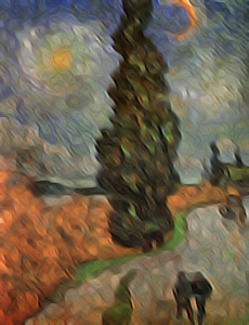
In **Figure 2** the diffusivity was computed on a grayscale version of the color image. Then it was applied
to each color channel individually in order to use the anisotropic smoothing
filter on color images, a more stringent analysis of the topic is given in [#weickert1999].
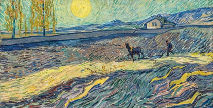
a) Original.
b) Video transition.
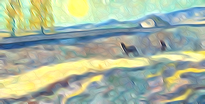
c) Final result.
**Figure 2:** _Filtering of the van Gogh painting "Enclosed Wheat Field with Ploughman". The video in the middle transforms from the unfiltered image on the left to the filtered image on the right._
Comparing the different stencils
-------------------------------------------------------------------------------
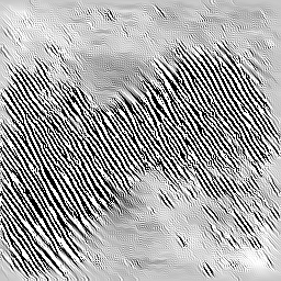
The main motivation behind using more accurate difference approximations is a reduction
in artifacts and improved stability of the filter. These artifacts can to some extent be observed
in **Figure 3** where the Kroon based method performs much better than the other three.

a) Original.

b) Finite differences.

c) Sobel.
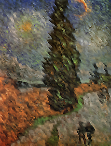
d) Scharr.
e) Kroon.
**Figure 3:** _Filtering of the van Gogh painting "Road with Cypress and Star" (Cypres bij sterrennacht). **a)** The finite difference filtered image has some severe artifacts and is not very stable, shown after 40 iterations. **b and c)** The Sobel and Scharr filtered images, both after 100 iterations, show some checkerboard artifacts also described in the papers by Kroon. **d)** Finally the Kroon filtered image, shown after 500 iterations, has a more desirable result and is more stable._
Artifacts and instability
========================================================================
Unlike the [isotropic linear and nonlinear](../image_smoothing_by_nonlinear_diffusion) diffusion filters
I encountered a lot more problems with different artifacts showing up in the results for
the anistropic diffusion. The checkerboard artifacts, visible both in **Figure 3 and 4**, were
adressed by using the kernels by Kroon. However a more severe artifact I often encountered was
due to an instability where the filter starts to enhance noise in such a way that the result
completely loses any resamlance of the original image, such as in **Figure 4 c**.

a) Original.
b) Video transition.
c) Noisy result.
**Figure 4:** _The anisotropic filter was sometimes sensitive to noise and artifacts. The result was computed with the Scharr kernels for 400 iterations, other settings was the same as for Figure 1. The fingerprint image is taken from [#weickert1998]._
Conclusion
========================================================================
Anisotropic, nonlinear, image filtering is a powerful image processing technique that
can be used to smooth the image content while preserving its structure.
However I found it was much more difficult to find parameters that gave satisfying
results compared to the [isotropic nonlinear smoothing](../image_smoothing_by_nonlinear_diffusion). It was also more sensitive with regards
to generating artifacts by enhancing noisy features.
The nonlinear smoothing has essentially one parameter that modulates the influence
of local contrast on the diffusivity. The implemented anisotropic filter had four parameters.
Gaussian smoothing of the image with standard deviation $\sigma$, Gaussian smoothing of the diffusivity tensor
with standard deviation $\rho$, $\alpha$ which modulates the coherence enhancing and $C$
which modulates the edge enhancing, although only one of these last two is applied at a time.
On top of this several differentiation stencils was tested.
I found the influence of these parameters on the final result not very intuitive and I
would probably have benefited greatly from a GPU implementation together witha GUI
for real time inspection of the results.
Although the results I got was not exactly what I had hoped for it was a good
mathematical exercise and I will continue to experiment and hopefully write
a 3D implementation as well.
+++++
**Bibliography**:
[#aubertkornprobst2006]: Aubert G. and Kornprobst P. 2006
**_Mathematical problems in image processing: Partial Differential equations and the calculus of varations._**
2nd edition.
https://link.springer.com/book/10.1007/978-0-387-44588-5
[#farid2004]: Farid H. and Eero P. S. 2004.
**_Differentiation of discrete multidimensional signals._**
IEEE Transactions on image processing 13.4 (2004): 496-508.
DOI: https://doi.org/10.1109/TIP.2004.823819
https://ieeexplore.ieee.org/abstract/document/1284386
[#kroon2009numerical]: Kroon D.J. 2009.
**_Numerical optimization of kernel based image derivatives._**
Short Paper University Twente
http://www.k-zone.nl/Kroon_DerivativePaper.pdf
[#kroon2009coherence]: Kroon D.J. _et al_. 2009.
**_Coherence filtering to enhance the mandibular canal in cone-beam CT data._**
IEEE-EMBS Benelux Chapter Symposium, volume 11, number 10.
https://ris.utwente.nl/ws/portalfiles/portal/5459986/Kroon_CoherenceFiltering.pdf
[#kroon2010optimized]: Kroon D.J. _et al_. 2010.
**_Optimized Anisotropic Rotational Invariant Diffusion Scheme on Cone-Beam CT._**
Medical Image Computing and Computer-Assisted Intervention – MICCAI 2010, vol. 6363.
DOI: https://doi.org/10.1007/978-3-642-15711-0_28
http://link.springer.com/10.1007/978-3-642-15711-0_28.pdf
[#kroon2010toolbox]: Kroon D.J. 2010.
**_Image edge enhancing coherence filter toolbox_**
Retrieved march 2, 2022
https://www.mathworks.com/matlabcentral/fileexchange/25449-image-edge-enhancing-coherence-filter-toolbox
[#weickert1998]: Weickert J. 1998.
**_Anisotropic diffusion in image processing._**
Teubner Stuttgart
http://www.lpi.tel.uva.es/muitic/pim/docus/anisotropic_diffusion.pdf
https://www.mia.uni-saarland.de/weickert/Papers/book.pdf
[#weickert1999]: Weickert J. 1999.
**_Coherence-enhancing diffusion of colour images._**
Image and Vision Computing, vol. 17, no. 3–4, pp. 201–212
DOI: https://doi.org/10.1016/S0262-8856(98)00102-4
https://www.sciencedirect.com/science/article/abs/pii/S0262885698001024
[#weickert2002]: Weickert J. & Scharr, H. 2002.
**_A scheme for coherence-enhancing diffusion filtering with optimized rotation invariance._**
Journal of Visual Communication and Image Representation, 13(1-2), 103-118.
DOI: https://doi.org/10.1006/jvci.2001.0495
https://www.sciencedirect.com/science/article/abs/pii/S104732030190495X?via%3Dihub
https://madoc.bib.uni-mannheim.de/1837/1/2000_04.pdf
[#wiki]: **_Diffusion equation_**
https://en.wikipedia.org/wiki/Diffusion_equation
[#sobel]: Sobel I. _et al_. 2014.
**_History and definition of the so called Sobel-operator, more appropriatly named the Sobel-Feldman Operator._**
https://www.researchgate.net/profile/Irwin-Sobel/publication/285159837_A_33_isotropic_gradient_operator_for_image_processing/links/5af73f41aca2720af9cf6063/A-33-isotropic-gradient-operator-for-image-processing.pdf
Code for all figures and examples:
https://bitbucket.org/nils_olovsson/diffusion_image_filters/src/master/